A Hypothesis That Has Been Tested Again and Again With Similar Results Each Time Is

Learning Outcomes

• Under appropriate conditions, acquit a hypothesis examination virtually a divergence between 2 population means. State a conclusion in context.

The Hypothesis Test for a Divergence in Ii Population Means

The general steps of this hypothesis examination are the aforementioned as always. As expected, the details of the atmospheric condition for use of the test and the test statistic are unique to this test (only similar in many ways to what nosotros have seen before.)

Step 1: Determine the hypotheses.

The hypotheses for a difference in two population ways are similar to those for a difference in two population proportions. The null hypothesis, H₀, is once more a argument of "no effect" or "no difference."

• H₀: μ₁ – μ₂ = 0, which is the aforementioned every bit H₀: μ₁ = μ₂

The alternative hypothesis, H_a, can be any one of the following.

• H_a: μ_one – μ_two < 0, which is the same as H_a: μ₁ < μ₂
• H_a: μ₁ – μ₂ > 0, which is the same every bit H_a: μ₁ > μ₂
• H_a: μ₁ – μ_two ≠ 0, which is the same as H_a: μ₁ ≠ μ₂

Footstep 2: Collect the data.

As usual, how nosotros collect the data determines whether nosotros can use it in the inference procedure. We have our usual two requirements for information collection.

• Samples must exist random to remove or minimize bias.
• Samples must exist representative of the populations in question.

We use this hypothesis exam when the data meets the post-obit conditions.

• The 2 random samples are independent.
• The variable is normally distributed in both populations. If this variable is non known, samples of more than than 30 will have a difference in sample means that can be modeled fairly past the t-distribution. As nosotros discussed in "Hypothesis Test for a Population Mean," t-procedures are robust even when the variable is non ordinarily distributed in the population. If checking normality in the populations is impossible, and then we look at the distribution in the samples. If a histogram or dotplot of the data does not testify extreme skew or outliers, we take it as a sign that the variable is not heavily skewed in the populations, and nosotros use the inference procedure. (Note: This is the aforementioned status we used for the ane-sample t-test in "Hypothesis Test for a Population Mean.")

Footstep iii: Appraise the evidence.

If the conditions are met, then we calculate the t-exam statistic. The t-test statistic has a familiar form.

[latex]T\text{}=\text{}\frac{(\mathrm{Observed}\text{}\mathrm{difference}\text{}\mathrm{in}\text{}\mathrm{sample}\text{}\mathrm{means})-(\mathrm{Hypothesized}\text{}\mathrm{departure}\text{}\mathrm{in}\text{}\mathrm{population}\text{}\mathrm{ways})}{\mathrm{Standard}\text{}\mathrm{error}}[/latex]

[latex]T\text{}=\text{}\frac{({\stackrel{¯}{x}}_{ane}-{\stackrel{¯}{ten}}_{2})-({μ}_{1}-{μ}_{2})}{\sqrt{\frac{{{s}_{1}}^{two}}{{northward}_{1}}+\frac{{{s}_{2}}^{ii}}{{northward}_{2}}}}[/latex]

Since the zip hypothesis assumes there is no difference in the population means, the expression (μ_ane – μ₂) is ever zero.

As we learned in "Estimating a Population Hateful," the t-distribution depends on the degrees of freedom (df). In the one-sample and matched-pair cases df = n – 1. For the ii-sample t-test, determining the right df is based on a complicated formula that we practise not embrace in this course. We volition either give the df or use engineering to find the df. With the t-test statistic and the degrees of freedom, we tin utilise the appropriate t-model to find the P-value, just as we did in "Hypothesis Test for a Population Mean." We can even utilise the same simulation.

Step 4: Country a conclusion.

To state a determination, nosotros follow what we take done with other hypothesis tests. Nosotros compare our P-value to a stated level of significance.

• If the P-value ≤ α, we reject the nix hypothesis in favor of the alternative hypothesis.
• If the P-value > α, we fail to reject the goose egg hypothesis. We do non have enough show to support the alternative hypothesis.

As always, we state our conclusion in context, usually by referring to the alternative hypothesis.

Example

"Context and Calories"

Does the visitor you lot keep bear on what y'all eat? This example comes from an article titled "Bear on of Group Settings and Gender on Meals Purchased past College Students" (Allen-O'Donnell, One thousand., T. C. Nowak, Thousand. A. Snyder, and Thou. D. Cottingham, Journal of Applied Social Psychology 49(ix), 2011, onlinelibrary.wiley.com/doi/x.1111/j.1559-1816.2011.00804.ten/full). In this study, researchers examined this outcome in the context of gender-related theories in their field. For our purposes, we wait at this research more narrowly.

Footstep 1: Stating the hypotheses.

In the article, the authors make the following hypothesis. "The attempt to appear feminine will be empirically demonstrated by the purchase of fewer calories by women in mixed-gender groups than past women in aforementioned-gender groups." We translate this into a simpler and narrower research question: Practise women purchase fewer calories when they eat with men compared to when they eat with women?

Hither the ii populations are "women eating with women" (population ane) and "women eating with men" (population ii). The variable is the calories in the meal. We test the post-obit hypotheses at the 5% level of significance.

The null hypothesis is ever H₀: μ₁ – μ₂ = 0, which is the same as H₀: μ₁ = μ₂.

The alternative hypothesis H_a: μ₁ – μ₂ > 0, which is the same as H_a: μ_ane > μ_two.

Here μ₁ represents the mean number of calories ordered by women when they were eating with other women, and μ_ii represents the hateful number of calories ordered past women when they were eating with men.

Note: It does not matter which population we label as 1 or 2, but once we decide, we accept to stay consistent throughout the hypothesis test. Since we expect the number of calories to be greater for the women eating with other women, the difference is positive if "women eating with women" is population 1. If you prefer to work with positive numbers, cull the group with the larger expected hateful equally population 1. This is a good general tip.

Pace 2: Collect Information.

Equally usual, there are 2 major things to keep in mind when considering the collection of data.

• Samples need to be representative of the population in question.
• Samples need to be random in order to remove or minimize bias.

Representative Samples?

The researchers state their hypothesis in terms of "women." We did the same. But the researchers gathered data by watching people eat at the HUB Rock Café II on the campus of Indiana Academy of Pennsylvania during the Jump semester of 2006. Almost all of the women in the data ready were white undergraduates between the ages of eighteen and 24, so at that place are some definite limitations on the scope of this study. These limitations will affect our conclusion (and the specific definition of the population means in our hypotheses.)

Random Samples?

The observations were nerveless on February xiii, 2006, through February 22, 2006, between 11 a.chiliad. and vii p.thousand. Nosotros can meet that the researchers included both lunch and dinner. They too made observations on all days of the week to ensure that weekly client patterns did non confound their findings. The authors state that "since the fourth dimension flow for observations and the place where [they] observed students were limited, the sample was a convenience sample." Despite these limitations, the researchers conducted inference procedures with the information, and the results were published in a reputable journal. We will too conduct inference with this data, but nosotros besides include a discussion of the limitations of the written report with our conclusion. The authors did this, also.

Do the information met the conditions for utilize of a t-examination?

The researchers reported the following sample statistics.

• In a sample of 45 women dining with other women, the average number of calories ordered was 850, and the standard difference was 252.
• In a sample of 27 women dining with men, the average number of calories ordered was 719, and the standard divergence was 322.

One of the samples has fewer than xxx women. We need to brand sure the distribution of calories in this sample is not heavily skewed and has no outliers, simply we do not have admission to a spreadsheet of the actual data. Since the researchers conducted a t-test with this data, we volition assume that the conditions are met. This includes the assumption that the samples are independent.

Pace three: Assess the evidence.

Every bit noted previously, the researchers reported the following sample statistics.

• In a sample of 45 women dining with other women, the boilerplate number of calories ordered was 850, and the standard deviation was 252.
• In a sample of 27 women dining with men, the average number of calories ordered was 719, and the standard deviation was 322.

To compute the t-examination statistic, brand sure sample 1 corresponds to population i. Here our population ane is "women eating with other women." So x ₁ = 850, s _i = 252, n ₁ =45, and then on.

[latex]T\text{}=\text{}\frac{{\stackrel{¯}{x}}_{1}\text{}\text{−}\text{}{\stackrel{¯}{x}}_{2}}{\sqrt{\frac{{{s}_{ane}}^{2}}{{due north}_{i}}+\frac{{{s}_{ii}}^{2}}{{n}_{ii}}}}\text{}=\text{}\frac{850\text{}\text{−}\text{}719}{\sqrt{\frac{{252}^{2}}{45}+\frac{{322}^{2}}{27}}}\text{}\approx \text{}\frac{131}{72.47}\text{}\approx \text{}ane.81[/latex]

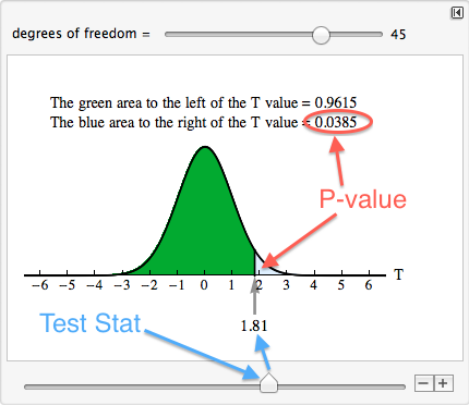
Using applied science, we determined that the degrees of freedom are virtually 45 for this data. To detect the P-value, we use our familiar simulation of the t-distribution. Since the alternative hypothesis is a "greater than" statement, we look for the area to the right of T = ane.81. The P-value is 0.0385.

Step 4: State a decision.

Generic Determination

The hypotheses for this test are H₀: μ₁ – μ₂ = 0 and H_a: μ₁ – μ₂ > 0. Since the P-value is less than the significance level (0.0385 < 0.05), nosotros reject H₀ and accept H_a.

Decision in context

At Indiana University of Pennsylvania, the mean number of calories ordered past undergraduate women eating with other women is greater than the mean number of calories ordered by undergraduate women eating with men (P-value = 0.0385).

A Comment about Conclusions

In the decision above, we did not generalize the findings to all women. Since the samples included only undergraduate women at 1 academy, we included this information in our determination. Just our decision is a cautious statement of the findings. The authors encounter the results more than broadly in the context of theories in the field of social psychology. In the context of these theories, they write, "Our findings support the assertion that repast size is a tool for influencing the impressions of others. For traditional-age, predominantly White higher women, diminished meal size appears to be an try to assert femininity in groups that include men." This viewpoint is echoed in the following summary of the written report for the general public on National Public Radio (npr.org).

• Both men and women appear to choose larger portions when they consume with women, and both men and women cull smaller portions when they eat in the company of men, co-ordinate to new research published in the Periodical of Applied Social Psychology. The study, conducted among a sample of 127 college students, suggests that both men and women are influenced by unconscious scripts about how to bear in each other'southward company. And these scripts alter the style men and women consume when they eat together and when they swallow apart.

Should we be concerned that the findings of this study are generalized in this way? Perhaps. But the authors of the article address this concern past including the post-obit disclaimer with their findings: "While the results of our research are suggestive, they should be replicated with larger, representative samples. Studies should be washed not merely with primarily White, eye-form college students, merely as well with students who differ in terms of race/ethnicity, social class, age, sexual orientation, and so forth." This is an case of expert statistical practice. It is oftentimes very difficult to select truly random samples from the populations of interest. Researchers therefore discuss the limitations of their sampling design when they discuss their conclusions.

In the post-obit activities, yous volition accept the opportunity to practise parts of the hypothesis examination for a difference in 2 population means. On the adjacent folio, the activities focus on the entire process and also incorporate engineering science.

Endeavor It

National Wellness and Nutrition Survey

munozrookencepor.blogspot.com

Source: https://courses.lumenlearning.com/wmopen-concepts-statistics/chapter/hypothesis-test-for-a-difference-in-two-population-means-1-of-2/

Share this post